Introduction to Quantum computing
When opening IBM's Quantum Computing page we see "Tomorrow’s computing, today". For me, this is a great way to show newcomers what quantum computing really means today. I'm no expert in quantum mechanics, I don't even know enough to the extent of explaining how it works to someone. But one thing I know is that we are in a similar phase as Engineers and Computer Scientists were in the '40s or '50s, developing the first classical computers. I don't believe that quantum computers can fully replace our classical ones, but they surely will have a major role in our lives in the future, and we are just at the beginning.
I won't explain how quantum computers work, but I recommend watching the video below, from Kurzgesagt – In a Nutshell. It's a 7-minute video and does a great job comparing quantum computers with classical ones, so if you are completely new to this matter, you should take the time to watch it, also.
You might have heard about NPC (NP-Complete) problems, if not, the Wikipedia page makes a good summary with some examples. Why am I talking about these problems? A NP problem is very hard to answer with our current technology and could take years if not centuries to reach an answer.
That's where the Monte Carlo algorithm comes in! It is a computation process that uses random numbers to produce an outcome. So, if there is a procedure for verifying whether the answer given by a Monte Carlo algorithm is correct, and the probability of a correct answer is bounded above zero, then with probability one running the algorithm repeatedly while testing the answers will eventually give a correct answer.
At the moment of writing this blog post, we only achieved quantum supremacy two times. Quantum supremacy is when a quantum computer outperforms a classical one. The goal of this blog post is not to enter into details, but you can read more here about the last time this has been achieved. And even more recently, Quantum Algorithms cracked nonlinear equations, by first "disguising" them as linear ones (more here).
In finance, problems like portfolio evaluation, personal finance planning, risk evaluation, and derivatives pricing are good examples of applications to Monte Carlo methods.
Nevertheless, Monte Carlo methods have a problem. If we want to obtain the most probable outcome of a wide distribution or obtain a result with a very small associated error, the required number of simulations can be stratospheric.
Quantum Amplitude Estimation (QAE) algorithm is a quantum-accelerated Monte Carlo algorithm. QAE can sample a probabilistic distribution quadratically faster than the next best classical method, allowing it to estimate expectation values extremely efficiently.
To know more about these particular methods and how to use them in financial problems, check this post from the Quantum World Association.
Financial Businesses and Quantum
According to IBM, here, "25% of small- and medium-sized financial institutions lose customers due to offerings that don’t prioritize the customer experience." and "It is estimated that financial institutions are losing between USD 10 billion and 40 billion in revenue a year due to fraud and poor data management practices."
Quantum computers can run whole-market simulations better in finding patterns, performing classifications, and making predictions that are not possible today with classical computers.
JPMorgan Chase wants to be ready for the quantum leap. The company has an unofficial leader, with the task to build a “quantum culture”, trying to discover how quantum computing can change the financial industry.
Barclays first started to explore quantum computing in 2017 and concluded that quantum computing’s potential was so great that they should commit to an initial program of research and development.
And we have many other cases to add to these ones.
Programming Quantum Computers
There are various approaches at the moment, to program a quantum computer. Microsoft has developed Q# programming language, IBM has Qiskit, a Python package, etc.
These are still in an early stage compared with what we can achieve with classical programming languages. Nevertheless, the road ahead seems promising.
Coding the first quantum circuit
IBM offers a Circuit Composer. It's a graphical quantum programming tool that lets you drag and drop operations to build quantum circuits and run them on real quantum hardware. You can check some instructions on how to use it here.
This Circuit Composer should look like the following screenshot.
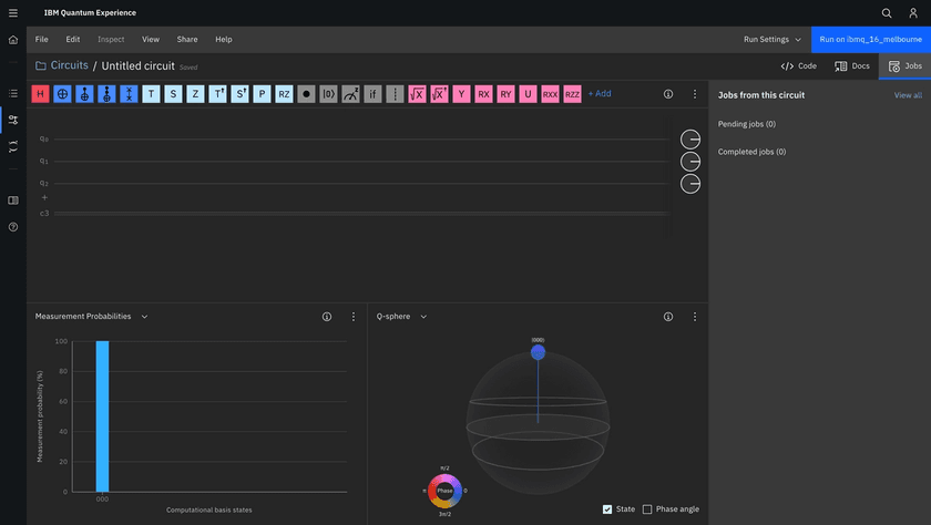
In this blog post, we will follow the IBM tutorial and develop a Bell State as a "Hello World" circuit.
A Bell State is defined as a maximally entangled quantum state of two qubits. This means that if Alice and Bob held an entangled qubit, and Alice measured her qubit the outcome would be perfectly random, with either possibility having a probability of 1/2. But if Bob then measured his qubit, the outcome would be the same as the one Alice got. So, to Bob, at first sight, he would also get a random outcome, but if Alice and Bob communicated they would find out that, although the outcomes seemed random, they were correlated.
Step 1 - Add an H gate (Hadamard gate) to your circuit q[0].
The Hadamard gate acts on a single qubit. It maps the basis state of the qubit to have equal probabilities to become 1 or 0 (i.e. creates a superposition).
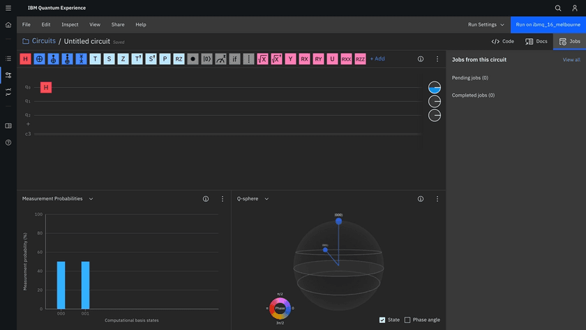
To add a gate to your circuit, drag and drop the operation from the palette of quantum operations to the top qubit, q[0].
Step 2 - Add a controlled-NOT gate to your circuit.
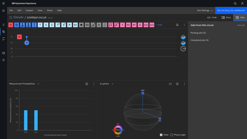
Controlled gates, such as controlled-NOT gate (or CNOT or CX) act on 2 or more qubits, where one or more qubits act as a control for some operation. For example, the CX acts on 2 qubits and performs the NOT operation on the second qubit only when the first qubit is |1⟩, otherwise leaves it unchanged.
To add a CX gate to your circuit, drag and drop the operation from the palette of quantum operations to the right of the gate. This operation acts on two qubits.
Step 3 - Add a measurement operation.
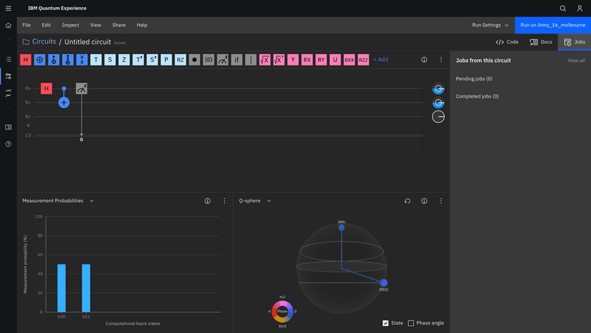
To add a measurement to your circuit, drag and drop the measurement operation from the palette of quantum operations to the right of the CX operation.
The measurement result is recorded as a classical bit on the classical register. The vertical wire connecting the measurement operation to the bottom wire depicts information flowing from the qubit down to the classical register.
Run the job and analyze results
You have now built your first quantum circuit. The visualization panels below your circuit give a simulated result that updates automatically as you add and remove operations. But you can also run the job in one real quantum computer, by clicking the top right corner button. It is possible to configure some settings, like system, provider, or shots (the number of times to run the code). Running jobs can take some time, depending on the number of jobs in the queue, so be prepared for that.
Therefore, most of the time is sufficient to just observe the simulation results. By looking at Measurement Probabilities, we can conclude that the final state of our little circuit has a 50% chance to be |000> or |001>.
However, looking at the real result, the probabilities are not 50%. This is caused by noise and all sorts of technology limitations at the moment.
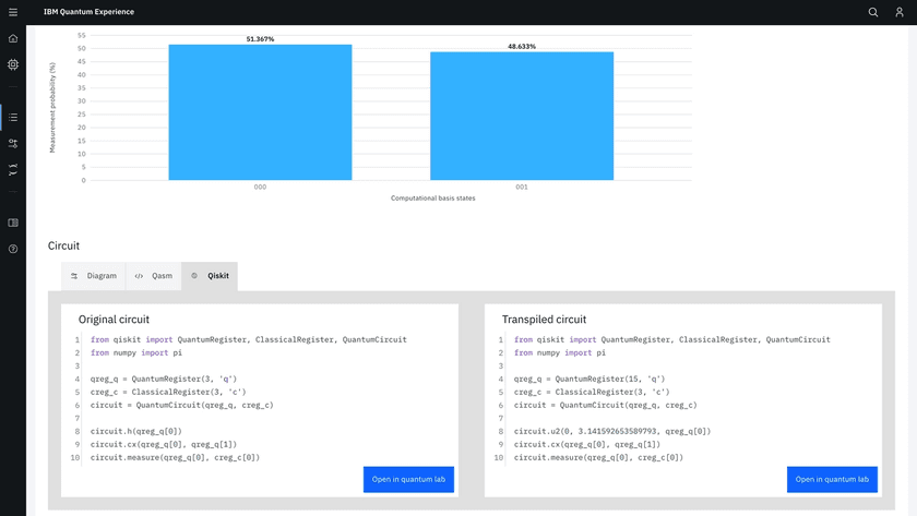
It is also possible to check the code version of the circuit we created.
More complex tutorials
There are more complex circuits as tutorials, such as the Grover's algorithm. It is a search algorithm, that can speed up an unstructured search problem quadratically. Here you can find a brief explanation and the respective final circuit.
In the same guide from IBM, there is also a link to some Jupyter Notebooks, including Financial Tutorials. Continuing on the thread of increasing effort from classical Banks and Financial Institutions on the theme, you may want to experiment with the Credit Risk Analysis.
Wrapping up
Quantum computing is a very interesting and promising topic, and we at Finiam are going to be attentive to new signs of progress that can impact the world.
See you around!